Common Misconceptions about Hierarchical Generative Models (Part 2 of 3)

By Richard D. Lange ca. March 2019

Archival note: this is a post recovered from Richard's old grad-school blog "Box and Arrow Brain." References to 'recent' things are relative to 2019, references to 'the lab' mean the Haefner Lab at UR, and information may generally be outdated.

In the previous post I discussed my first 2 of 7ish not-quite-true or misleading intuitions about hierarchical generative models. If you haven't read it yet, start there. This post picks up where the other left off.

Background: priors, average-posteriors, and linear Gaussian models

The ideas in this post all rely on a distinction between a model's prior and its average posterior. I find this distinction so conceptually fundamental that I'm giving it its own section here.

Linear Gaussian Image Models

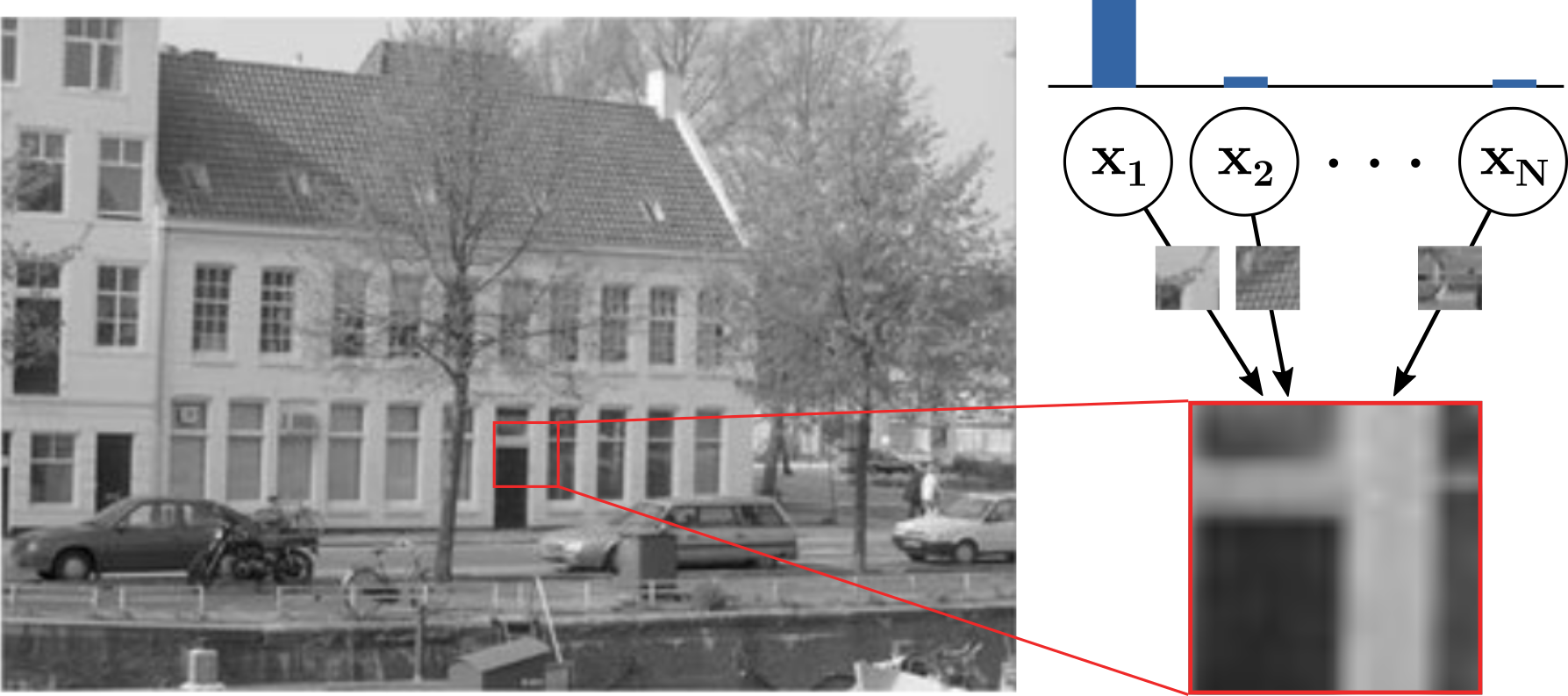
As a motivating example, consider the classic sparse linear Gaussian model used by vision researchers everywhere, and let's start with just a single layer of latent variables. In the generative direction, images are generated as a noisy sum of features, where the features are selected so that each image only has a few of them present (a sparse prior). Inference corresponds to finding which subset of features are present in a given image. $\begin{aligned} x & \sim p (x) \\ I & = η + \sum_{i} A_{i} x_{i} \end{aligned}$ Where $η$ is noise added to the pixels and $A_{i}$ is the image patch corresponding to feature $x_{i}$ . If we have $N$ features and $P$ pixels per image, then $x \in R^{N}$ and each $A_{i} \in R^{P}$ . This is sometimes written as a matrix vector product where $A$ is a $P \times N$ matrix, so that $\sum_{i} A_{i} x_{i} = Ax$ .

To ensure that only a few features are present in each image, $p (x)$ is set to be a sparse prior. In other words, most of the $x$ s are zero most of the time. One simple to do this is with the prior $p (x) \propto e^{- \sum_{i} | x_{i} |^{α}}$

This is visualized in the following figure. The signature of a spare prior is mass concentrated along the axes of the space, since these are the regions where only one feature is "active" and the rest are near zero.

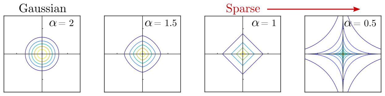
When $α = 2$ this is the familiar Gaussian prior. We get sparseness when $0 < α \leq 1$ .

Now, let's say we choose a value of $α$ that gives us a sparse prior and fit the image patches $A$ to data using Maximum Likelihood. Intuitively, this means we want to find a collection of image patches where any given image is well-described as the sum of a small number of them. A seminal result in vision science is that when such a model is fit to natural images, the learned features begin to look like the kinds of visual features that drive neurons in V1^[1].

In the sparse linear Gaussian model, each small image patch in a dataset is modeled as the weighted sum of features. The sparse prior encourages only a few $x$ s to explain each image. The result is that, once fit to data, the model’s $A_{i}$ s (the features visualized on each arrow on the right) tend to pick out recurring image parts like edges, corners, gradients, etc, loosely resembling the kinds of things neurons in V1 seem to care about.

Maximum Likelihood as distribution matching

I mentioned Maximum Likelihood as a way to "fit" the $A$ s to data. Maximum Likelihood chooses the parameters of a model for which the data that we see is most likely to have been generated by the model with those parameters. There's a nice connection between this idea of finding the parameters for which each image is most likely and the idea of fitting the distribution of images. Recall that the marginal likelihood of a model is the distribution over its outputs that you get by averaging over all possible assignments to other variables: $p (I; A) = \int p (I | x; A) p (x) d x$ Another way to view Maximum Likelihood learning is making the marginal likelihood as close as possible to the actual data distribution. To see why, we will to use Kullback-Leibler (KL) divergence, which is a common mathematical tool for quantifying how dissimilar two probability distributions are. Intuitively (but, it turns out, not formally), KL is like the "distance" between two distributions -- it has the desirable properties that it is zero only when the two distributions are exactly equal, and it gives a positive value otherwise. It also just so happens that KL divergence is not symmetric (one of the reasons it's not formally admissible as a "distance" measure), so we write that the divergence "from p to q" is $K L (p | | q) = \int p (I) \log \frac{p (I)}{q (I)} d I$

A reasonable goal when fitting a generative model to data is that the marginal likelihood of the model should match the empirical data distribution. In other words, we should seek to minimize the distance (e.g. measured using KL) between two distributions: the marginal likelihood and the data distribution. But, we don't have access to the data distribution itself, only a dataset images sampled from it. Conveniently, KL has the form of an expected value, so it can be estimated using samples from $p$ : $\begin{aligned} K L (p | | q) & = \int p (I) \log \frac{p (I)}{q (I)} d I \\ = E_{p} [\log \frac{p (I)}{q (I)}] \\ \approx \frac{1}{D} \sum_{i = 1}^{D} \log \frac{p (I_{i})}{q (I_{i})}, I \sim p \\ = \frac{1}{D} \sum_{i = 1}^{D} \log p (I_{i}) - \log q (I_{i}) \\ = - \frac{1}{D} \sum_{i = 1}^{D} \log q (I_{i}) + c o n s t, I \sim p \end{aligned}$ If $q$ is the model we're trying to fit to some given data, we simply ignore the $\log p$ term, since nothing we change in the model will affect it. Returning to our goal of fitting a model by matching marginal likelihood to the data distribution, we see now that minimizing KL is equivalent to minimizing the sum of $- \log q$ for all of our data points, which is just another way of saying maximizing the likelihood of q!

If you take nothing else away from this post, remember this: when we fit a generative model to data, we're at best getting the marginal likelihood close to, but not equal to to the data distribution (at worst, there are bugs in the code and/or we get stuck in local optima). A sparse linear Gaussian model is in fact a terrible model of what images actually look like and its marginal likelihood will not look like real image patches. Still, we can try fitting the model to a dataset of natural images using Maximum Likelihood to get as close as possible under the restrictive assumptions that the world is sparse, linear, and Gaussian.

Priors and Average-Posteriors

The rules of probability define a “loop” from the prior p(x) to images (or data more generally) p(I) and back again. Inference and generation are mirror images. I call this “Bayes’ Loop”. The next figure describes how this symmetry falls apart in practice.

So what does this digression on divergence and model-fitting have to do with priors and posteriors? Well, when we fit a model to some data that does a poor job of capturing the actual data distribution (i.e. the KL between the data distribution and marginal likelihood remains high), some elementary rules in probability seem to break down. Take the definition of marginalization, which tells us that $p (x) = \int p (x, I) d I$ , and the product rule which tells us that $p (x, I) = p (x | I) p (I)$ . Putting these together, we get $p (x) = \int p (x | I) p (I) d I$ In plain English, this says that the prior $p (x)$ is equal to the average posterior (each $p (x | I)$ is one posterior, and the average is taken over many images $p (I)$ ). The trouble is, this is only true if we use a self-consistent definition of all of the probabilities involved. It's tempting to replace the integral over $p (I)$ here with an expected value using the data as we did for KL above, but this is not allowed if $p_{d a t a} (I) \neq p (I; A)$ , which is almost certainly the case for any model of real data!

There are essentially two different probabilistic models at play, one defined by the generative direction, and one defined by the inferences made on a particular dataset. This is visualized in the next figure. The key point is that in any realistic setting, the chosen "prior" will not equal the "average posterior," even after fitting with Maximum Likelihood. In fact, one could reasonably argue that the average posterior is a better definition of the prior than the one we started out with!

On the left in blue is our generative model, and on the right in green is what I’ll call the inference model. Unlike in the previous figure, the two sides are distinct and don’t form a closed loop. “Fitting a model” means adjusting the p(I|x) term until the marginal likelihood (lower left) is as close as possible to the data distribution (lower right). In any nontrivial setting, there will be some error $ϵ$ — some part of the data that our model is unable to capture. As long as there is some $ϵ$ at the bottom, there will be some $η > 0$ error at the top, between the regularizer r(x) and the average posterior q(x). Confusion abounds when in some contexts the “prior” means r(x), and in other contexts it means q(x)! I am deliberately not writing “p(x)” from now on to keep these ideas separate.

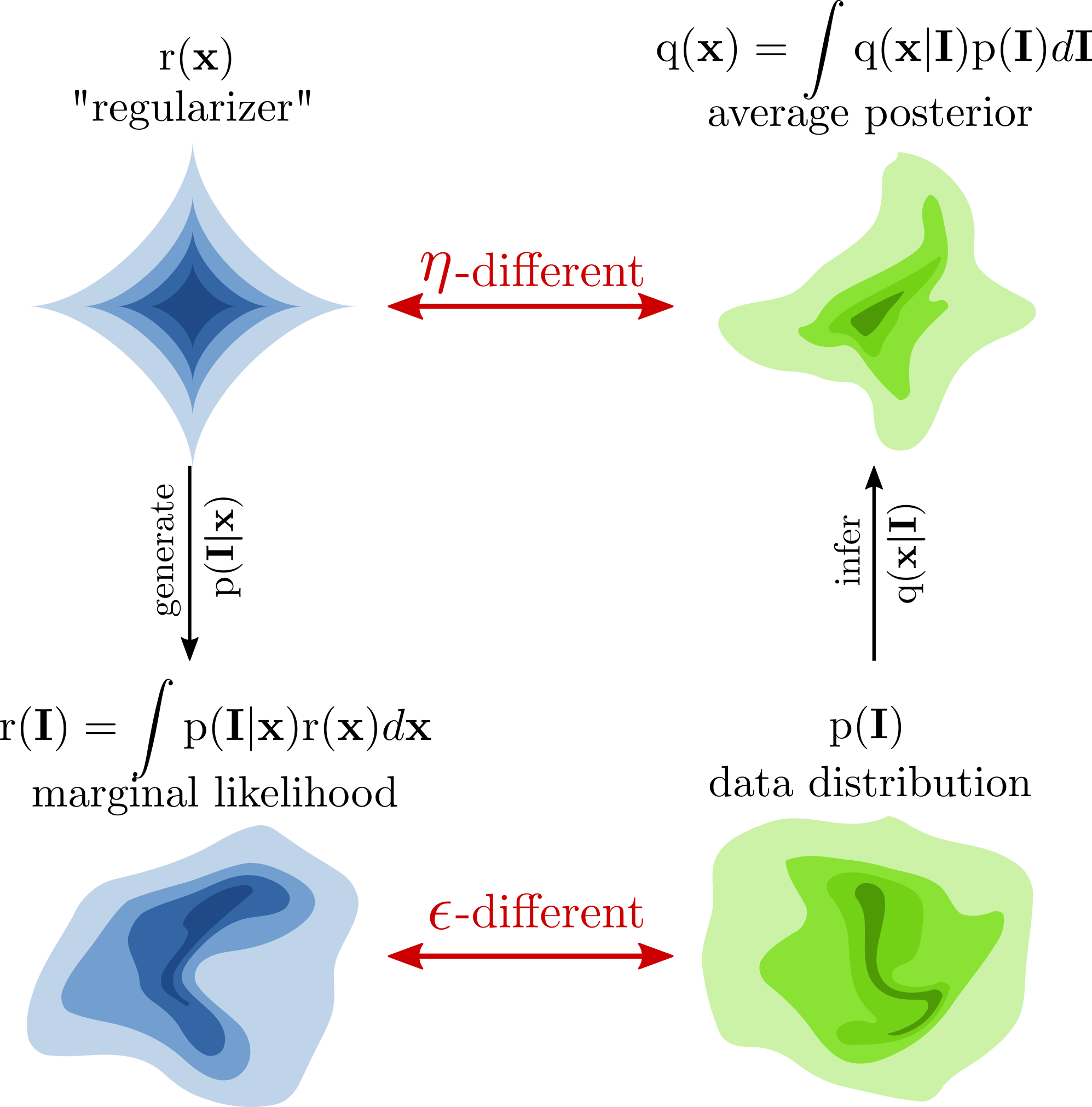
With the figure above as a reference, let's define the following terms:

r(x) is what I've so far called the "prior" -- the distribution on x we choose before fitting the model. It really should be called the regularizer (hence my choice of "r"). During fitting, it guides the model towards using some parts of x and away from others, but does not by itself have any real guarantees.
p(I|x) is the part that does the generating. When x is given, we can use it to sample an image. When I is given, it defines the likelihood of x. Importantly, this term is the "glue" which connects the generative model on the left to the inference model on the right.
r(I) is the distribution of images we get when we sample x from r(x) and I from p(I|x): $r (I) = \int p (I | x) r (x) d x$
p(I) is the "true" distribution of images. We never have access to the distribution itself, but typically have a dataset of samples from it. Having a dataset sampled from p is like having a $ρ$ that approximates p as a mixture of delta distributions: $p (I) \approx ρ (I) = \frac{1}{N} \sum_{i = 1}^{N} δ (I - I_{i})$
q(x|I) is the "pseudo-posterior" we get when we use p(I|x) as the likelihood and r(x) as the prior.^[1] It's "pseudo" since, in some sense, r(x) isn't really a prior! (More on this in a moment). The pseudo posterior is defined using Bayes' rule with the "r" model (in other words, it's the inference we would make if we assumed that r(x) was the correct prior): $q (x | I) = \frac{r (x) p (I | x)}{r (I)}$
q(x) is the "average pseudo-posterior" on the dataset: $q (x) = \int p (I) q (x | I) \approx \frac{1}{N} \sum_{i = 1}^{N} q (x | I_{i})$ .

With this foundation in mind, let's move ahead to the three main misconceptions of this post. But first, here are two bonus thoughts based on the above:

Imagine generating new data by first selecting x then choosing I conditioned on x. Sampling x from the regularizer will result in images that do not look like the data, while if we first sample x from the average posterior, they will. Zhao et al (2016) used an analogous argument when they showed that alternately sampling from images and from the first layer of a hierarchical model is sufficient to samples all images^[2], though they concluded from this that hierarchical models are in some sense fundamentally broken (a nice derivation but hasty conclusion IMHO).
Estimates of mutual information are inflated when comparing each data point's posterior to the regularizer, rather than comparing each posterior to the average posterior. This is only half of the reason why I have βeef with β-VAEs^3-4^, which will hopefully be the subject of a future post.

Intuition 3: the prior is a free parameter

Now it's really time to get to today's common misconceptions.

Selecting the regularizer r(x) is one of many design choices for a model. For instance, I described above how some sparse coding models begin by selecting $α$ to define a level of sparseness.

During fitting, the regularizer r(x) only acts as a guide, encouraging but not enforcing a distribution on the latents. For nearly all intents and purposes, the average pseudo-posterior q(x) is a better use of the term "prior" than r(x). While not perfect, q(x) is in some sense "closer" to obeying the rules of probability and Bayes' Loop than r(x). Importantly, q(x) is determined as much by the likelihood p(I|x) and data distribution p(I) as it is by r(x). So while the choice of regularizer r(x) is free, the resulting "prior" we get back after fitting a model is not. Unfortunately, computing q(x) and expressing it concisely is not possible in general, so it's not uncommon to see the assumption that $q (x) \approx r (x)$ in papers, but this is an assumption that needs to be verified!

In principle, we could try to fit the prior to data as well. Imagine that we begin with a regularizer r(x), then over the course of learning we adjust it to better match the average posterior q(x). Each new r(x) defines a new q(x), which we then use to update r(x). When the dust settles and the model converges, we hope to arrive at a "self-consistent" model where the regularizer matches the average posterior -- the rare case where both r(x) and q(x) are promoted to the status of "prior." Three things can go wrong with this approach: first, there is a degenerate solution where r(x) converges to a point. Congratulations! The prior equals every posterior, but the model is useless. This can be addressed by cleverly restricting the degrees of freedom of r. Second, we are always forced to select some parameterization of r(x), and there is no guarantee that q(x) can be expressed in a chosen parametric family of distributions. There will almost always be some lingering mismatch. Third, we may thus opt for an extremely flexible family of r(x) only to find that results are less interpretable. Sparse priors are popular in part because they are interpretable. Super powerful semi-parametric models generally aren't (see any paper using "normalizing flows" to define the prior^5-6^). Depending on your goals in a given context, of course, this may be an acceptable trade-off.

Intuition 4: complicated priors imply complicated posteriors

In a well-calibrated model, the prior is equal to the average posterior. Each individual posterior per input (per image, e.g.) may be simple and easy to express, while taken collectively they map out a prior that is complex.

The sparse linear Gaussian model, in addition to being mathematically "nice" to analyze and implement, has the property that when it is fit to natural images, the individual latent features tend to pick out small oriented edges, much like the sorts of low-level visual features picked up by canonical V1 neurons.

Even if we ignore for a moment that a model with sparse sums of oriented edges doesn't capture the distribution of natural images well, we can appreciate the difficulty in describing the prior for all the ways in which edges naturally co-occur -- in extended lines, in curves, in textures, all of these possibly contiguous for long distances even behind occluders. Any reasonable prior for low-level visual features like edges is going to be complicated. Pseudo-posterior inference with a sparse prior is already hard enough, so the existence of a complicated prior surely makes the problem truly intractable, right?

Not necessarily! In the figure above to the right, I've sketched a cartoon to visualize how complicated priors may arise from simple posteriors. Think of it this way -- edges may co-occur in images in complex ways, but when was the last time this kept you from seeing a particular edge in a particular image?

(Another way to say this is that inference with a complicated prior is only hard when the likelihood is uninformative, since the posterior is then more similar to the prior. When the likelihood is informative, the posterior is more similar to the likelihood, as in typical well-lit viewing conditions of natural scenes.)

Intuition 5: complicated posteriors imply complicated priors

The reverse of the previous point can happen as well. Not only do complicated priors not necessarily imply complicated posteriors, but many complicated posteriors may conspire to fit together, summing to a simple prior!

“Complicated” posteriors may, in principle, sum up to result in a simple prior like the pieces of a puzzle, each with an irregular shape, fitting together to form a simpler whole.

If this visualization seems contrived, just think of what happens in the sparse linear Gaussian model with $0 < α < 1$ that has "explaining away" (e.g. the classic "overcomplete" models). The prior is "simple" by design -- it has one parameter and is unimodal. Each individual posterior is in general multi-modal as the same image may be described as the sum of different of subsets of features. Following the logic of Bayes' Loop, all of these multi-modal posteriors must necessarily sum to give us back the simple prior!^[2]

Footnotes

Writing q(x|I) may also call to mind approximate inference methods, since even computing the pseudo-posterior as described above may be intractable. In this case, it's natural to define q(x|I) as the approximation, and q(x) as the average-approximate-pseudo-posterior.
What I'm calling Bayes' Loop describes a useful diagnostic tool that a generative model and inference algorithm are implemented correctly. If it's all implemented correctly, then you should be able to draw samples $x_{i} \sim r (x)$ and use them to create a pseudo dataset $I_{i} \sim p ({I | x}_{i})$ . If the average posterior $q (x | I_{i})$ (or average sample from the different posteriors) doesn't match r(x), there must be a bug!

References

Olshausen, B. a, & Field, D. J. (1997). Sparse coding with an incomplete basis set: a strategy employed by V1? Vision Research.
Zhao, S., Song, J., & Ermon, S. (2016). Learning Hierarchical Features from Generative Models.
Higgins, I., Matthey, L., Pal, A., Burgess, C., Glorot, X., Botvinick, M. M., ... Lerchner, A. (2017). β-VAE: Learning Basic Visual Concepts with a Constrained Variational Framework. ICLR.
Alemi, A. A., Fischer, I., Dillon, J. V, & Murphy, K. (2017). Deep Variational Information Bottleneck. ICLR, 1--19.
Rezende, D. J., & Mohamed, S. (2015). Variational Inference with Normalizing Flows. ICML, 37, 1530--1538.
Kingma, D. P., Salimans, T., & Welling, M. (2016). Improving Variational Inference with Inverse Autoregressive Flow. Advances in Neural Infromation Processing Systems, (2011), 1--8.