Common Misconceptions about Hierarchical Generative Models (Part 3 of 3)

By Richard D. Lange ca. July 2019

Archival note: this is a post recovered from Richard's old grad-school blog "Box and Arrow Brain." References to 'recent' things are relative to 2019, references to 'the lab' mean the Haefner Lab at UR, and information may generally be outdated.

This post is the last in a series on misconceptions or not-quite-right intuitions about hierarchical generative models, their pertinence to perception, and their relevance to representations. This post explicitly builds on the foundations of the previous two, so I highly suggest reading Part 1 and Part 2 if you haven't yet!

Intuition 6: it all boils down to simple priors, self-consistency, and marginal likelihoods

By now, I hope you appreciate that fitting a latent variable model to data is difficult, especially if you desire certain guarantees. The kinds of things you might want out of your model are

1. High marginal likelihood. The model should fit the data it has already seen, in the sense that existing data points should be likely to be generated by sampling from the model.
2. Generalization. The model should also place high probability on hypothetical future data it hasn't seen but plausibly could. This alone is a topic for a future post or two. I'll largely ignore it here (which is reasonable in the case of large amounts of data with good coverage).
3. Self-consistency. New data sampled from the model should look like real data, and inferences made on real data should be consistent with the prior. Using the terminology introduced in Part 2, we can say that the prior $p(\mathbf{x})$ should equal the average posterior $q(\mathbf{x})=\frac{1}{N}\sum _{n=1}^{N}p(\mathbf{x}|{\mathbf{y}}_n).$ One caveat, with generalization in mind, is that the average posterior really ought to take into account unseen future data too, but generalization is again a topic for the future.
4. A simple prior. Simple priors tend to be more interpretable, for some non-technical definition of both "simple" and "interpretable." For instance, a "sparse" prior means that each data point or image can be explained by a small subset of all possible latent features.

Most of Part 2 was devoted to explaining the tensions between high marginal likelihood, self-consistency, and simple priors. These are by no means trivial criteria to meet, but let's move on from those difficulties for now. Let's say I hand you on a silver platter a dataset of interest $\mathbf{Y}$ and a generative model $\mathbf{x}\to \mathbf{y}$ that meet all four of the above desiderata. That is, I give you a definition of latents $\mathbf{x}$, prior $p(\mathbf{x})$, and generating procedure $p(\mathbf{y}|\mathbf{x})$ where the prior is simple, the model is self-consistent, and the dataset is big enough that we won't even worry about generalization. Are we done? Can we go home?

As you may have guessed by now, the answer is: not necessarily. Meeting the four criteria above ensures that we have a good statistical model of the data distribution and can synthesize new, realistic-looking samples. If you skim the current literature on deep generative models (GANs and VAEs, mostly), you might get the impression that synthesizing photo-realistic images of faces and cheeseburgers is the ultimate goal of these research programs. More often, synthesizing artificial data is intended as a proxy for testing whether the model has learned and internalized something about the data -- whether it has developed good representations.

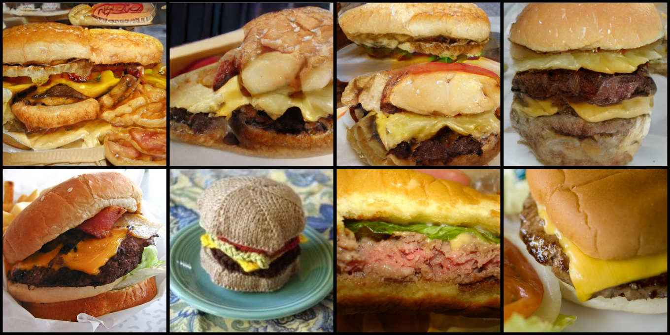
I'm here today to tell you that despite Feynman's famous quote about understanding, generating better images does not necessarily translate to understanding the content of those images.

What I cannot create, I do not understand

Richard Feynman

What's a cheeseburger?

GANs

The remainder of this post is essentially another elaborate way of saying that representation matters. (Spoilers, I know). To build intuitions towards that conclusion, though, we need a digression to define and visualize Mutual Information.

Digression: Mutual Information and KL Divergence

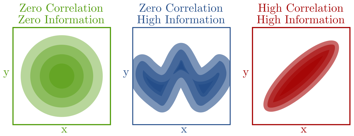
Mutual Information is a way to quantify how related or dependent two random variables are on each other. It goes far beyond correlation, picking up on any and all linear and nonlinear statistical dependencies between two variables, and each of those variables can be as low- or high-dimensional as you like.

Formally, Mutual Information between $\mathbf{X}$ and $\mathbf{Y}$ is defined as $$\mathcal{I}[\mathbf{X},\mathbf{Y}]=\sum _{\mathbf{x}\in \mathbf{X}}\sum _{\mathbf{y}\in \mathbf{Y}}p(\mathbf{x},\mathbf{y})\log \frac{p(\mathbf{x},\mathbf{y})}{p(\mathbf{x})p(\mathbf{y})}$$

An intuitive way to rewrite this is as a Kullback-Liebler (KL) divergence from the joint distribution $p(\mathbf{x}\mathbf{,}\mathbf{y})$ to the product of marginal distributions $p(\mathbf{x})p(\mathbf{y})$: $$\begin{array}{rl}\mathcal{I}[\mathbf{X},\mathbf{Y}]& ={\mathbb{E}}_{p(\mathbf{x},\mathbf{y})}[\log \frac{p(\mathbf{x},\mathbf{y})}{p(\mathbf{x})p(\mathbf{y})}]\\ & =KL(p(\mathbf{x},\mathbf{y})||p(\mathbf{x})p(\mathbf{y}))\end{array}$$

Recall that KL is something like the "distance" between two distributions in that it is zero when its two arguments are exactly equal, and positive otherwise. This helps build some intuitions -- it means that mutual information is zero when-and-only-when the joint distribution $p(\mathbf{x}\mathbf{,}\mathbf{y})$ is equal to the product of marginal distributions $p(\mathbf{x})p(\mathbf{y})$. The more intricacies exist in the joint distribution that cannot be predicted from the marginals alone, the higher the information.

Another way we can think of mutual information is as saying, "how much do I learn about the values of x when I observe some value of y (or vice versa)?" If after observing y you can't make any more precise predictions for y than the prior you started with, then we'd conclude that x and y are independent, i.e. $p(\mathbf{x}|\mathbf{y})=p(\mathbf{x})$. This would imply $p(\mathbf{y}\mathbf{,}\mathbf{x})=p(\mathbf{x}|\mathbf{y})p(\mathbf{y})=p(\mathbf{y})p(\mathbf{x})$, so the joint equals the product of marginals, the KL is zero, and the information between x and y is nil. On the other hand, if observing x constrains plausible values of y in some way, then x contains information about y (and vice versa).

Especially when thinking in terms of latent variable models and inference, I find it even more insightful to rewrite mutual information like this: $$\begin{array}{rl}\mathcal{I}[\mathbf{X},\mathbf{Y}]& =\sum _{\mathbf{x}\in \mathbf{X}}\sum _{\mathbf{y}\in \mathbf{Y}}p(\mathbf{x},\mathbf{y})\log \frac{p(\mathbf{x},\mathbf{y})}{p(\mathbf{x})p(\mathbf{y})}\\ & =\sum _{\mathbf{x}\in \mathbf{X}}\sum _{\mathbf{y}\in \mathbf{Y}}p(\mathbf{x}|\mathbf{y})p(\mathbf{y})\log \frac{p(\mathbf{x}|\mathbf{y})p(\mathbf{y})}{p(\mathbf{x})p(\mathbf{y})}\\ & =\sum _{\mathbf{y}\in \mathbf{Y}}p(\mathbf{y})\sum _{\mathbf{x}\in \mathbf{X}}p(\mathbf{x}|\mathbf{y})\log \frac{p(\mathbf{x}|\mathbf{y})}{p(\mathbf{x})}\\ & ={\mathbb{E}}_{p(\mathbf{y})}[KL(p(\mathbf{x}|\mathbf{y})||p(\mathbf{x})]\end{array}$$

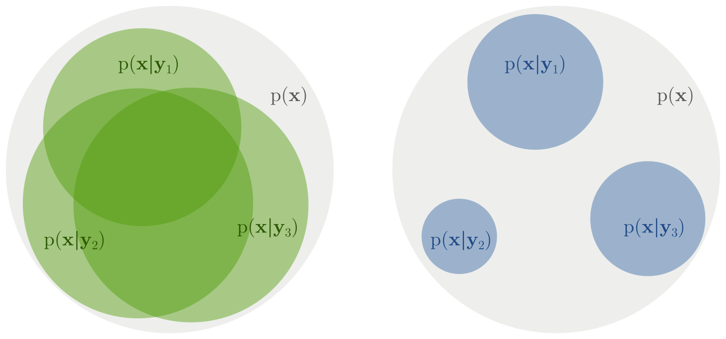
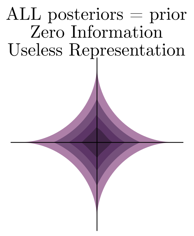
This says that we can think of mutual information as the expected KL (over all y) between the posterior on x and the prior on x. This has always been the most intuitive way of thinking about mutual information for me. If giving me a y tells me nothing about x, then the posterior equals the prior and the information is zero. This form also suggests a nice visualization of what it means to have low or high mutual information: in the low information case, each individual posterior on x is "close" to the prior, while in the high information case each posterior differs drastically from the prior. Combining this with some of the ideas from the previous post, we also know the average of all of posteriors must also be equal to the prior in all cases.

Insight 6a: Mutual Information is necessary for representation learning

With that digression for definitions out of the way, we can return to the problem of assessing the $\mathbf{x}\to \mathbf{y}$ model. The question was: is it enough to say we have a "good" or "useful" model of the data y if we fit the data with a self-consistent model that has a simple prior on x (in other words, matching criteria 1-4 above)? Let's make this concrete with an example.

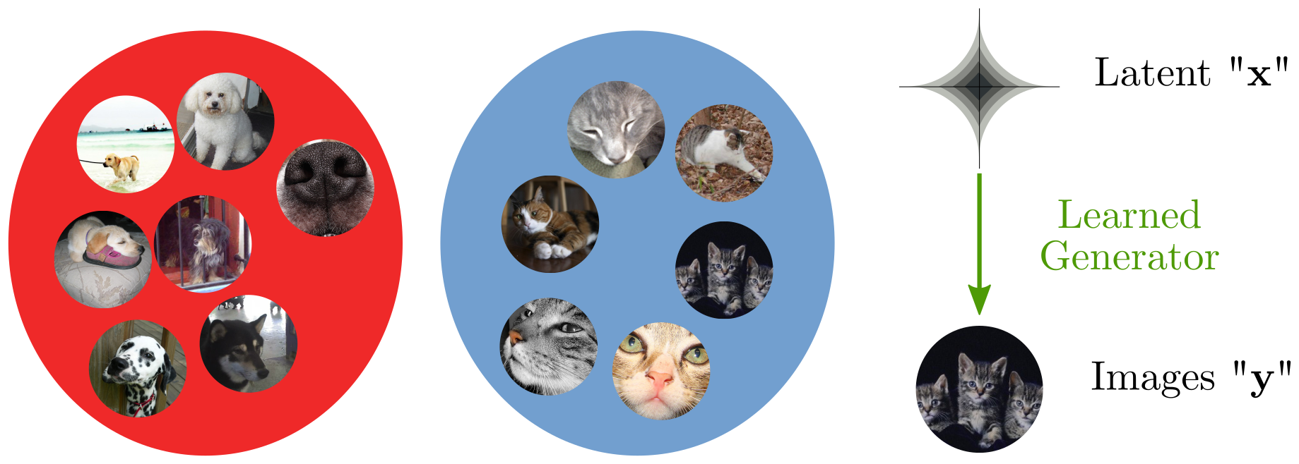
Returning to the classics, let's say we want to represent the content of some images with some continuous latent variables, and in particular, we're interested in distinguishing images of cats from images of dogs, but we won't allow ourselves to see the category labels during learning. You are provided with the following dataset:

So, you build a latent variable model that has a nice, interpretable sparse prior on the latents, hoping that ${\mathbf{x}}_1$ will capture "dog features" and ${\mathbf{x}}_2$ will capture "cat features." The sparse prior encourages the model towards representations with only one critter per image.

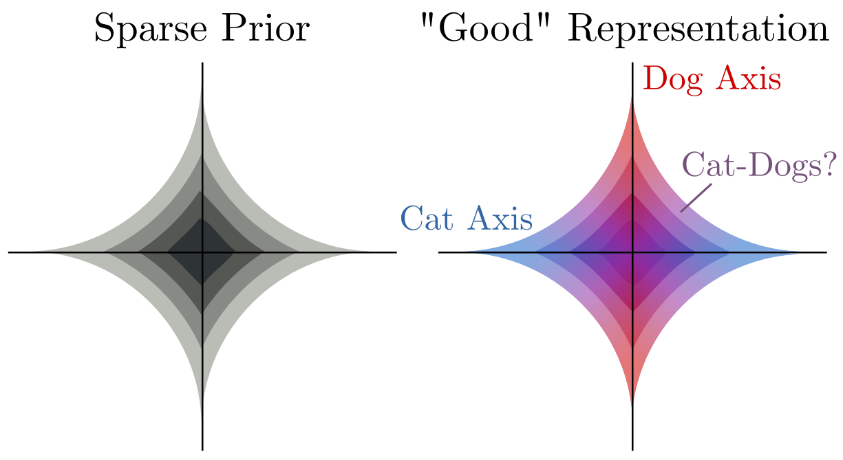
If all we do is train this model using Maximum Likelihood (ML) or its approximate cousin, maximizing the Evidence Lower BOund or ELBO, we get no guarantees that the latents will come to represent anything meaningful or useful!

Let's take a step back. In general, it's an incredibly intuitive and good idea to model complex data (like images) as byproducts of the hidden machinations of simpler processes. Pixels are complicated, high-dimensional, and just plain messy, but latent variables tell their story: objects, lights, textures, and optics interacted in complicated ways to create those pixels. That's why those of us in the biz' gravitate towards latent variable models in the first place. We hope that enforcing a "simple prior" on our latents will make them interpretable and useful in the same way that objects, lights, and textures are an interpretable, useful, and actionable representation of an image.

Classic latent variable training objectives, like ML and ELBO, don't do this for free. The single best way I've seen this explained is this: ML is all about marginal distributions. You win the ML game if you match the marginal probability of the data, and you win the self-consistency game (point #3 above) if you match the marginal probability of the latents (i.e. the prior) with the average posterior. The key to latent variables being a good representation of data, on the other hand, is that those latents need to tell you something about the data. Latents and data must covary. In other words, mutual information between latents and data is necessary. It follows quite plainly that ML and its cousins are not sufficient for representation learning.

This insight is one of those ideas that is so obvious in hindsight that you might (if you're me) wonder why it took reading two papers^1,2^, someone else' blog post^[3], and more than one evening staring at a blank wall to understand it.

I suspect that the reason this is a difficult pill to swallow for some is that we are accustomed to thinking of the mechanism of a generative model as given to us in advance. The steps that took place between specifying some objects, lights, and textures and capturing some pixels were a fairly rigid and well-understood physical process that can be emulated by a good rendering engine. Ironically, that rigidity may make this a difficult process to learn directly from data, but that is beside the point here. The current trend in machine learning, as exemplified by both the VAE and GAN literature, is to jointly learn the relation between data and latents while learning a highly flexible mechanism for simulating data based on those latents. We run into trouble when the mechanisms become too flexible. Given enough power, the generating mechanism can get greedy -- it might get so good at generating data on its own that it doesn't even need your darn latents!

Insight 6b: Mutual Information not sufficient for representation learning

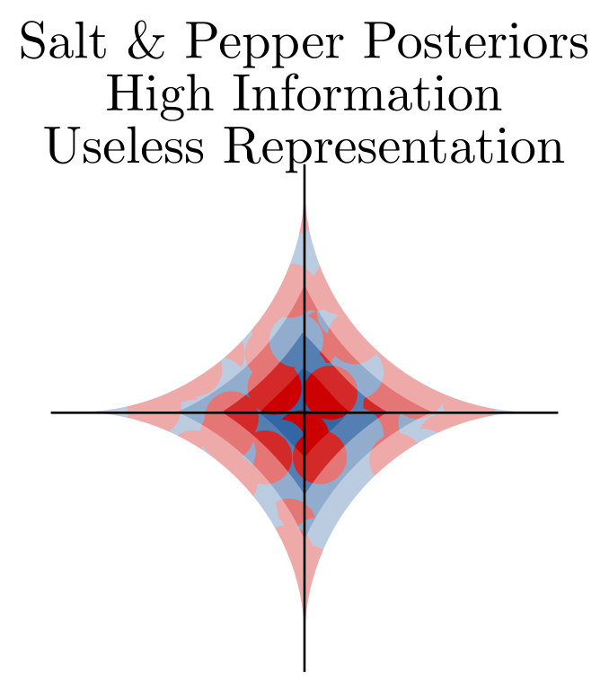
So, Mutual Information is at the very least a necessary part of a healthy relationship between latent variables and the modeled data. But is it enough? Well, take a look at the picture to the right, which I call the "salt and pepper posteriors" problem.

We get a self-consistent model that obeys the identities in "Bayes Loop" when the average of all posteriors equals the prior. We get high mutual information when each posterior is well-constrained by the data. As caricatured here, both of these can be satisfied while at the same time the latent space does absolutely nothing in terms of representing the original data in a more interpretable/useful/actionable form.

How to train your generative model

For starters, I highly recommend reading the references at the bottom of this post. These papers attack nearly all of the problems I've outlined here head-on, and do a much better job than I can do here discussing the inherent trade-offs between fitting a self-consistent model, fitting the data, and getting high mutual information with the latents. It turns out that we have our work cut out for us with these alone.

Still, these approaches will only get us about as far as "intuition 6a," but still leaves us with the "salt and pepper posteriors" problem in 6b. I'm convinced that in order to attack this problem -- to ensure that higher mutual information translates to better representations -- we need to step outside the current comfort zone of the field, where we take off-the-shelf arbitrarily-powerful generative models and derive newer and better training objectives until it looks good^[1]. Then again, the fact that I'm convinced of this may not say much -- perhaps in the future I'll be writing a post about how that intuition is misguided as well!

The key to unsupervised representation learning with generative models may (unsurprisingly?) be in building more rigid, domain-specific generative processes. The arbitrary power and flexibility of density networks (as used in VAEs and GANs) come with the price of fewer guarantees and fewer constraints, not all of which can be solved by bigger data.

Footnotes

1. In fact, Zhao et al (2018) essentially proved that the field has exhausted all possible options for fiddling with training objectives already! There's nothing left to do there. What genuinely puzzles me is why the authors called this a "negative result." Is it because, deep down, they hoped that off-the-shelf arbitrarily-powerful generative models were the path to effective unsupervised learning? Did they hope that enough cleverness in the loss function would lead to a breakthrough? I truly welcome differing opinions on the matter, but I choose to see this result as a win -- we now know that further progress will have to be made outside the realm of better loss functions! Great! Now we can close that door and focus on model architectures!

References

1. Alemi, A. A., Poole, B., Fischer, I., Dillon, J. V., Saurous, R. A., & Murphy, K. (2018). Fixing a Broken ELBO. http://arxiv.org/abs/1711.00464
2. Zhao, S., Song, J., & Ermon, S. (2017). InfoVAE: Information Maximizing Variational Autoencoders. http://arxiv.org/abs/1706.02262
3. https://www.inference.vc/maximum-likelihood-for-representation-learning-2/
4. Zhao, S., Song, J., & Ermon, S. (2018). The Information Autoencoding Family: A Lagrangian Perspective on Latent Variable Generative Models. Retrieved from http://arxiv.org/abs/1806.06514