The Blog of Why

By Richard D. Lange ca. December 2019

Archival note: this is a post recovered from Richard's old grad-school blog "Box and Arrow Brain." References to 'recent' things are relative to 2019, references to 'the lab' mean the Haefner Lab at UR, and information may generally be outdated.

Not long ago I read Judea Pearl's Book of Why to see what all the fuss on causality was about. I'm glad I did. It's one of those books that can so thoroughly change the way you look at certain problems that you forget what it was like thinking in different terms before. I'm pretty sure I used to think of "confounding" as a mysterious evil force that could call any result into question. Having understood "Backdoor Paths," confounding may still be evil but it is far less mysterious. Maybe even more importantly, the Book of Why drives home the point that there is no causality without assumptions, and that's OK! There had been, at least in my mind, an unspoken rule in statistics and machine learning that everything you need to know is in the data. Pearl and his causal colleagues grant us both the freedom and the necessary formalism to assume that smoke comes from fire, that the rooster crows because the sun rises, and that umbrellas do not cause the rain.

On the more technical side of things, the lab has been journal-clubbing chapters of The Elements of Causal Inference by Peters, Janzing, and Schölkopf. This book is full of beautiful mathematical results in their own right, but ironically, this book's emphasis on the technical definitions may leave the reader asking, "why?" The perspective on causality in Elements is an abstract and mathematical one. Just as you should hesitate to ask a mathematician for help with taxes or ask a theoretical computer scientist for tech support, Elements should be approached not for the practicality but for the theory. Readers interested in a primarily practical guide to causality for data analysis should read Mastering Metrics or Mostly Harmless Econometrics (neither of which I've read, but were recommended to me).

My goal with this post is to supplement and draw connections between Elements and BoW, but not replace either of them. I'll do my best to interpret why certain assumptions and presentation decisions were made in Elements, while giving some more intuitive visualizations in the spirit of BoW. Finally, I make a broad disclaimer that this post reflects my own best understanding of things, which is prone to mistakes. Comments and corrections are welcome!

On DAGs and Distributions

I first want to clear the air regarding the relationship between graphs and probability distributions. Formally, a Directed Acyclic Graph (DAG) is a set of vertices or nodes (V) and directed edges (E) such that there are no directed paths that form a cycle, or loop. Informally, a DAG is a bunch of circles (V) and arrows (E) where the nodes can be arranged in "left to right" order; a cycle would require doubling back from right to left.

So far, I've only described what a graph is. I've said nothing about random variables nor probability distributions. I'm asking you, dear reader, to set aside for a moment any experience you may have with graphical models such as Bayesian Networks or Markov Random Fields. Given some experience with these concepts, it's easy to forget that the graph and the distribution are separate objects. For instance, on the island of pure probability theory, random variables do not have "parents" or "children" -- these are graphical notions. Ideally we'll always find ourselves in situation that the properties of the graph (e.g. parent/child relations) agree with the properties of the distribution (e.g. statistical dependence), but this is not necessarily true.

Imagine that I give you a graph $G=(V,E)$ with $V=\{v_1,\dots ,v_N\}$ and a probability distribution $P(x_1,\dots ,x_N)$. Being the trickster that I am, I make no guarantees that these two things are related. You have some work to do say how and whether G and P are related. This is the easy-to-miss motivation behind the following definitions in Elements, chapter 6.5:

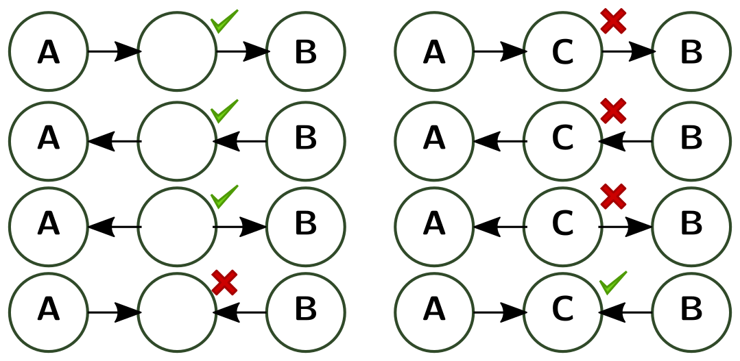
• d-separation is a property of the graph. Let A, B, and C be nodes in our graph -- see the above figure. Wherever there is a red "x," the path is blocked and we say A and B are "d-separated." You may recognize these diagrams as conditional dependence relations if you've seen Bayesian Networks before. But again, I emphasize that d-separation is a property of the graph, not of the distribution.
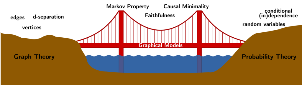
• A distribution P satisfies the Markov Property with respect to the graph G (or "P is Markovian with respect to G") if d-separation in the graph corresponds to independence in the distribution. If A and B are d-separated by C in the graph, it must be the case that A is independent of B given C in the distribution. Finally, we're starting to build bridges between G and P! There's a catch, though: the graph is allowed to have "too many" edges, since we made no claim for the converse: independence in P does not necessarily imply d-separation in G. In fact, there's a sort of "fully connected" G that vacuously satisfies the Markov Property for any joint distribution (see the figure on the left).
• There are two ways around this trivial solution. The direct converse to the Markov Property is called faithfulness. A distribution P is said to be faithful to the graph G if (conditional) independence in P corresponds to (conditional) d-separation in G. It simply flips the direction of the "if-then" implication of the Markov Property.
• The other way to deal with the vacuous solution of the Markov Property, Causal Minimality, directly attacks the superfluous edges. We say P is causally minimal with respect to G if P is Markovian with respect to G, but not with respect to any sub-graph of G. Just like that, we've explicitly ruled out the "too many edges" case: if you can delete an edge and still have the Markov Property, there were clearly too many edges.

Both Faithfulness and Causal Minimality "solve" the problem of the vacuous solution to the Markov Property, so it's tempting to think that they're equivalent. It turns out, however, that one can contrive edge cases (so to speak) where Faithfulness is violated despite the graph being Causally Minimal (example 6.34 in Elements). Emphasis on the "contrived-ness" of such examples. So while Faithfulness does turn out to imply Causal Minimality, the reverse is not true given some technicalities, but probably true in practice.

The authors of Elements are extremely careful not to conflate statements in the realm of graph theory ("there exists a path from node $v_i$ to $v_j$") with statements in the realm of probability ("random variables $x_i$ and $x_j$ are not independent"). But in building the bridge between them, it is easy for the reader to lose track. Take, for instance, the following notations found throughout the book: "$v_i{\text{⧸}\perp \perp }_G{v}_j$" expresses the graphical notion of the existence of a path (formally, "lack of d-separation"), while "$x_i\text{⧸}\perp \perp x_j$" expresses the probabilistic notion of dependence. It's easy to miss the subscripted "G," just as it's easy to forget that "d-separation" in a graph only tells you something about conditional independence in a distribution if the graph satisfies the Markov Property with respect to that distribution.

The Ladder of Causation

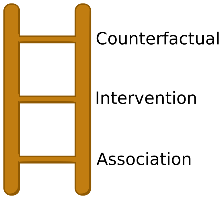
The most rudimentary form of statistical reasoning -- the lowest rung on the ladder -- is association. This rung is purely about observing correlations between variables, devoid of causal structure. We observe smoke concurrent with fire and umbrellas concurrent with rain. We reason abductively, "where there is smoke, there is probably fire," and we have no formal tools to distinguish this from "where there is fire, there probably is smoke," despite the common sense knowledge that there is an underlying causality $\text{fire}⟶\text{smoke}$.

Bayesian Networks (BN), despite their arrows, live at the observational level. The BN $\mathbf{x}⟶\mathbf{y}⟶\mathbf{z}$ does not mean there is a chain of causation from $\mathbf{x}$$to$\mathbf{z}$. Instead, the arrows (or, more to the point, the lack of arrows) in a BN signify statistical (in)dependencies. It's an instructive exercise to show that any joint distribution that can be written $p(\mathbf{x}\mathbf{,}\mathbf{y}\mathbf{,}\mathbf{z})=p(\mathbf{x})p(\mathbf{y}|\mathbf{x})p(\mathbf{z}|\mathbf{y})$ can be rewritten as $p(\mathbf{x}\mathbf{,}\mathbf{y}\mathbf{,}\mathbf{z})=p(\mathbf{z})p(\mathbf{y}|\mathbf{z})p(\mathbf{x}|\mathbf{y})$ without losing any information about the joint distribution of the three variables. The BN $\mathbf{x}⟶\mathbf{y}⟶\mathbf{z}$ is, in this sense, equivalent to $\mathbf{z}⟶\mathbf{y}⟶\mathbf{x}$ at the association level, which cares only about joint probability distributions.

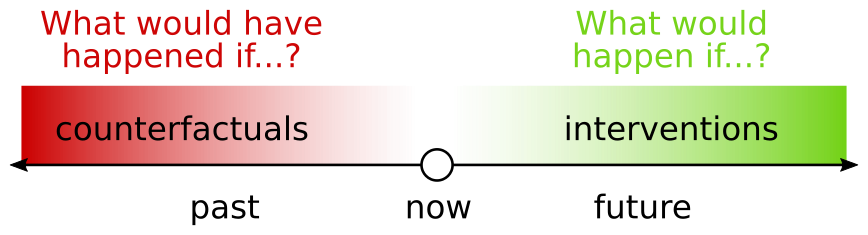
Moving up the ladder to interventions requires a simple but profound change: we endow the arrows of the BN with a direction. Such a model is aptly called a Causal Bayes Net (CBN). It's at this level that we distinguish between $p(\mathbf{y}|\mathbf{x}=x)$ and $p(\mathbf{y}|do(\mathbf{x}=x))$, the latter being known as the "do-operator". The first expression is the familiar Rung 1 statement, "what does observing that x has value $x$ tell me about y?" As before, this statement doesn't distinguish between $\mathbf{x}⟶\mathbf{y}$, $\mathbf{y}⟶\mathbf{x}$, or $\mathbf{x}⟵\mathbf{z}⟶\mathbf{y}$. The magic happens in $p(\mathbf{y}|do(\mathbf{x}=x))$, which can be read as the hypothetical question, "what would y be if I intervene to force x to have value $x$?".^[1] This "do-operator" respects the direction of the arrows: "do(x)" can propagate to y only if $\mathbf{x}⟶\mathbf{y}$ but not if $\mathbf{y}⟶\mathbf{x}$. Since the CBN formalism adds "do()" semantics but may still be used non-causally ($p(\mathbf{y}|\mathbf{x}=x$ rather than $p(\mathbf{y}|do(x=x))$), Pearl likes to say that Rung 2 of the ladder is strictly more powerful than Rung 1.

Though it may not seem like much here, moving from Rung 1 to Rung 2 -- from BNs to CBNs -- is a huge step. From what I can tell, the vast majority of causality research (and applications) live at Rung 2. First, the do-operator implies a certain agency in interacting with the data. Classical (Rung 1) statistics suffers from paralysis, dispassionately describing but unable to prescribe. Interventional thinking is necessary for anyone who acts in the world and wants to understand and predict the consequences of their actions. Furthermore, the second rung formalizes what it means for something to confound a measurement, and equips us with the necessary tools to deal with it. Finally, using the "do-calculus" we can sometimes circumvent the need for randomized controlled experiments and answer interventional questions using observational data (or prove they're unanswerable without such an experiment).

Interventions are about hypothetical questions, assuming some agency in changing the future course of history. Similarly, counterfactuals, as their name suggests, ask hypothetical questions "counter to the facts." Simply put, they are hypothetical questions about the past. Say you're playing a game of Backgammon.^[2] An interventional question would be, "what would happen if I capture the opponent's piece?" Interventions are clearly useful for planning. The comparable counterfactual question on some later turn would be, "what would have happened if I hadn't captured that piece?" The past being immutable, it seems at first glance that counterfactuals are good for nothing but regret.^[3] (More on this later). Further, it's not at all obvious at first why counterfactuals are more powerful (and require more assumptions) than interventions. These questions and more puzzled me upon first reading of BoW, later clarified somewhat in the formal arguments of Elements. But upon even further reflection, I confess I find myself once again puzzled about the definition and usefulness of counterfactuals. The points are subtle, so I will attempt to outline all of what I do and don't yet grasp about counterfactuals in the next few sections, perhaps sharing some of my puzzlement along the way!

Counterfactuals, SCMs, and all that

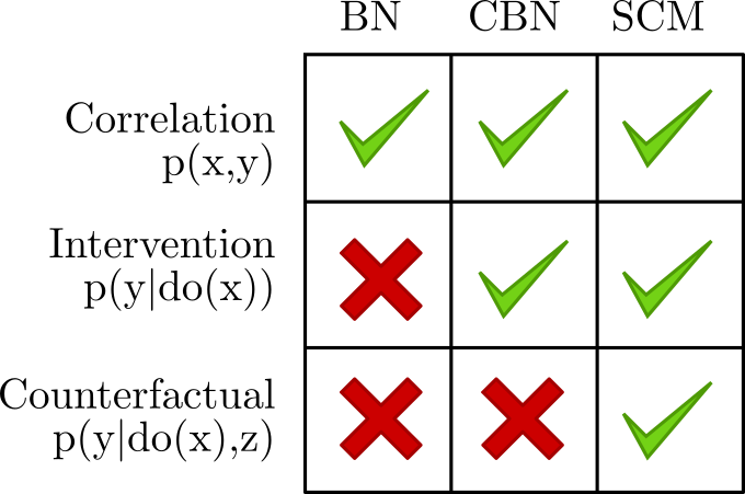
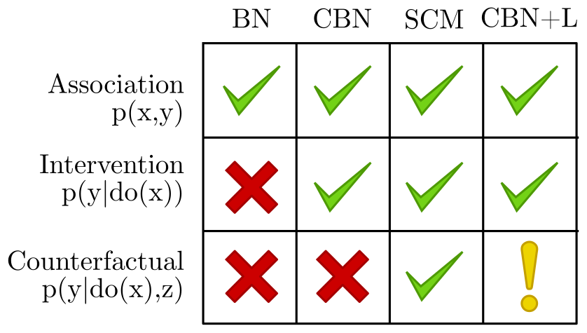
The Elements book wastes no time with Bayesian Networks nor their causal cousin, CBNs, jumping straight to Structural Causal Models (SCMs). If you'll excuse the shorthand notation, the table on the right suggests why: just as CBNs generalized BNs to move from Rung 1 to Rung 2, SCMs generalize both of them and add some functionality that we couldn't get before, namely counterfactuals.

Before defining what an SCM is, let's motivate it by trying (and failing) to answer a counterfactual question using the world's simplest CBN: $\mathbf{x}⟶\mathbf{y}$ with both variables taking on discrete values in $\{1,2,3,4\}$. We'll place a uniform prior on x, and say that y is always either equal to x or x+1 (wrapping around). All of this should be clear in the first panel of the following figure:

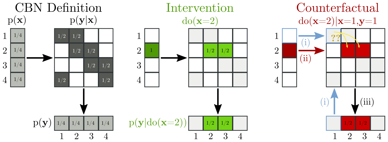
The left panel of this figure visualizes the x to y using a conditional probability table, mapping from the 4 values of x to the rows of the table, then to the 4 values of y. Entries of the table are normalized row-wise. The middle panel visualizes the intervention $do(\mathbf{x}=2$ as selecting a row of the table. The result is that y can only take on one of two values, each equally likely. So far so good for the CBN. We encounter trouble when we get to the counterfactual (right panel). I've graphically broken the counterfactual reasoning process down into three steps. First (i), an observation is made about the past, here it's observed that x and y had both been 1 (blue outlines). Given that information, we ask in the second step (ii), "what would have happened if x had instead been 2?" This is a problem of generalization -- we need to know what information from the observation that x and y were 1 would transfer to the case of x=2 (yellow arrows). The CBN simply has nothing to say about this transfer -- all we know is that y is chosen randomly given x. If no past knowledge transfers, the counterfactual question reduces to the interventional question, $p(\mathbf{y}|do(\mathbf{x}=2))$.

The trick of the SCM is to parameterize the randomness in $\mathbf{x}⟶\mathbf{y}$ by introducing an explicit noise variable which we'll call $\eta$ (the Greek letter "eta"). Having moved the randomness into $\eta$, y becomes a deterministic function of both x and $\eta$. For instance, we can recover the behavior of the above CBN with $$\begin{gathered} \eta \sim \{0,1\} \\ \mathbf{y}=\text{mod}(\mathbf{x}+\eta ,4), \end{gathered}$$ using the convention that mod() wraps around to 1. This is visualized in the SCM definition on the left, below:

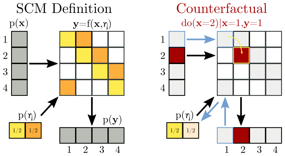
Interventional questions work exactly as in the CBN case before. Equipped with this new $\eta$ term in the SCM, something interesting happens in the counterfactual case: observing past values of both x and y now tells us something about $\eta$! Using the example from earlier, observing x=1**,y**=1 in the past tells us definitively that η must have been 0. Now, asking what would have happened if x had been 2, we can reason definitively that it would have resulted in y=2. By making the noise explicit, we now have information that transfers from one scenario to the other.

Lest this seem too easy, rest assured that there is no free lunch here. The above SCM is not the only one we could have constructed to match the initial CBN. Consider this one instead:

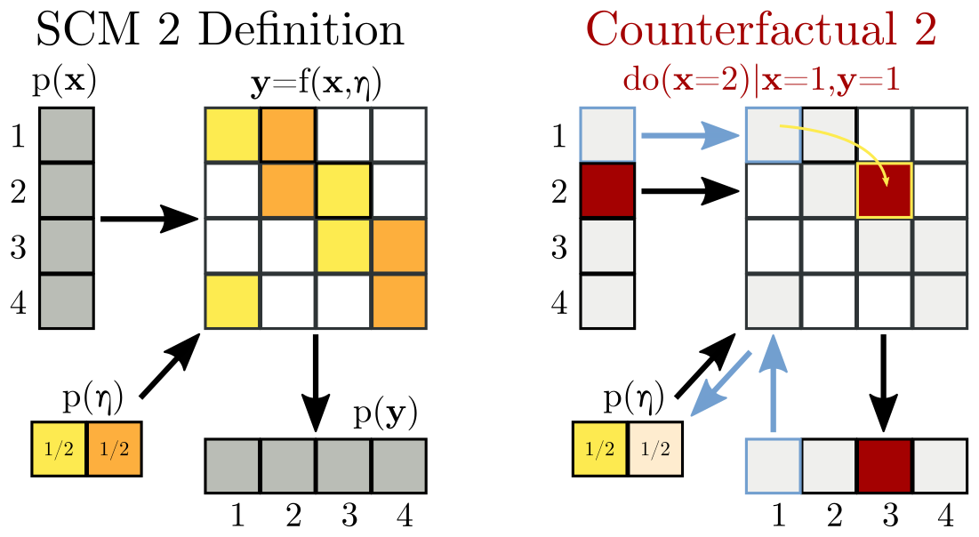
All I've done is exchange some yellows for oranges in the table. The original SCM and this SCM are interventionally equivalent -- they make exactly the same future predictions for any do(x) query! But, as is illustrated on the right, they give different counterfactual answers. Perhaps, then, you won't be surprised to learn that there are infinitely many SCMs consistent with a given CBN (all interventionally equivalent with each other), but the various SCMs are under no obligation to make similar counterfactual judgments.

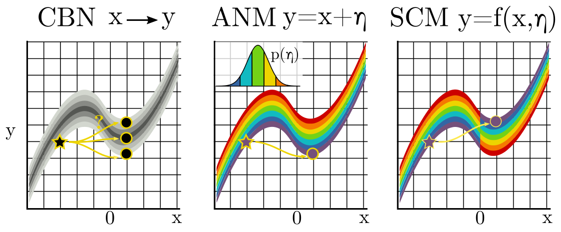
One can certainly argue that, in the above examples, the first SCM was "simpler" than the second. It could be defined using a single mod operation. Try writing an expression for the second SCM -- you'll find that is not nearly as concise. To the extent that SCMs describe reality, and to the extent that reality is simple, one way to select among them is by this criterion of simplicity. In the case of continuous variables, a "simple" SCM assumes that noise is simply additive. The following figure visualizes the exact same argument for continuous x and y:

Throughout this post, I've been carefully avoiding the phrase "counterfactual prediction," since to a scientist a prediction has the connotation of being something falsifiable. Pearl has argued that SCMs are, in fact, falsifiable since, loosely speaking, we might gain information in the future (for instance about a third variable "z") that tells us whether or not our judgments about the past had been correct. I confess I don't understand this argument. (To be fair, I can't say I've dug into it very deeply either.) Shouldn't any later information (z) that falsifies an SCM, by the principles of forward (interventional) prediction, falsify a CBN too? I hope the above diagrams make it clear that without further assumptions, no experiment (no intervention) can distinguish between interventionally-equivalent SCMs. For that, more assumptions will be needed...

I have another related confession of ignorance: despite all of the above, I don't understand why CBNs cannot be used for counterfactual reasoning. Both BoW and Elements make a similar case to the one I outlined above: if you don't make the noise explicit, you don't know how to transfer your knowledge about how the past was to hypothetical possibilities of how the past could have been. But here's my puzzle: what's the difference between making the noise, η, explicit, and introducing latent variables in the CBN formalism? What's the difference between the SCM $\mathbf{x}⟶\mathbf{y}⟵\eta$ where $\eta$ is noise and the CBN $\mathbf{x}⟶\mathbf{y}⟵\mathbf{w}$ where w is an unobserved latent variable? One answer is that the arrows in the SCM are all deterministic, but that's of course just a special case of a CBN using delta distributions for its conditional densities. Another answer is that the SCM formalism gives a private η to each variable (above, I could have been more precise by distinguishing ${\eta }_{\mathbf{x}}$ and ${\eta }_{\mathbf{y}}$), and all of these ηs are required to be a priori independent of each other. This makes a good amount of sense philosophically -- causally independent entities in the world don't share noise. But again, this is just a special case of the CBN with Latents (CBN+L). I think, reading Elements and BoW, it's easy to come away with the impression that SCMs are the one true path to counterfactual reasoning. But, realizing that η is just a highly constrained latent variable, it seems reasonable to me to adopt the CBN+L formalism as our framework of choice. (I can only infer myself that the CBN formalism is reserved for observed variables only, but I don't remember seeing this stated explicitly in Elements or BoW).

Are counterfactuals useful? A reinforcement-learning perspective

While there's no question that moving from association to intervention -- BN to CBN -- is useful, the utility of counterfactuals (CBNLs and SCMs) is far more subtle. Elements is an excellent introduction to the math of counterfactuals, but they don't tell the reader why they should care:

"Discussing whether counterfactual statements contain any information that can help us make better decisions in the future is interesting but lies beyond this work."

Elements, page 99

We humans really seem to love our counterfactual reasoning. We do it all the time. (As the joke goes, "Imagine a world without counterfactuals!"). It would be deeply puzzling if such a deeply human habit were spurious. So, how are counterfactuals useful? The common arguments are:

1. Counterfactuals ascribe credit or blame. Blame is used, for instance, in the legal system to determine guilt.
2. They help us learn to make a better decision next time we encounter a similar situation.
3. Counterfactual reasoning is necessary to falsify an SCM, or, equivalently, to learn the correct SCM.
4. Equipped with an incomplete or incorrect world model, a reinforcement learning agent will do better with counterfactual reasoning than with either interventional reasoning or pure replay.

Below, I will dive into each of these four arguments, but first a quick summary. I suspect that most readers will find (1) and (2) intuitive and familiar in virtue of, well, being human (no offense to web crawlers reading this). I will attempt to undo some of that intuition in a moment. Argument (3) likewise seems initially plausible, but of course, falsifying a model requires making measurements, and I'm not aware of any way to measure outcomes that, by definition, never happened. Finally, argument (4) is probably the most esoteric, but at the moment it's the only well-justified defense of counterfactuals I'm aware of. My goal here is to make the esoteric intuitive.

1. Counterfactuals are useful for ascribing credit and blame

Right off the bat, I'll make it clear that I don't deny this claim. It's practically tautological: credit goes to those without whom a goal would not have been accomplished. Somone is the target of blame when things would have been fine but for the decisions of that person. These definitions appeal directly to counterfactuals.

The issue is not with "credit" or "blame," but with the word "useful." To say that counterfactuals are useful because the assign credit and blame simply begs the question: what use is there in pointing fingers? Answers to this question generally fall into two categories: shaping future behavior and setting an example for others.

Let's say Alice discovers, to her horror, that someone has stolen the last cookie from the cookie jar. Bob sheepishly comes forward and admits to being the culprit. "It was in a rare moment of indulgence," he pleads, "it won't happen again!"

Alice reasons that the cookie would still be there, but for the actions of Bob, so she rightly blames him for the missing cookie. Now consider Bob's defense: "it won't happen again." If Alice accepts his defense at face value, there's nothing to be done. The cookie is gone now, and Bob will refrain from stealing future cookies. Great!

Still, Alice decides she had better be sure, so she punishes him by making him scrub the kitchen clean. She deters future wrongdoing by establishing a credible threat. Further, she knows that she needs to establish this threat so that other people won't take advantage of her kindness and steal her cookies in the future. Again, blame and deterrence ought to be viewed from the lens of what will happen next time.

As a quick side note, it hardly even feels like all the machinery of counterfactuals is necessary here, but the argument about "transferring the noise" earlier is, in fact, relevant! Our common sense is what allows us to imagine a "nearly identical" world in which Bob did not succumb to his desire for the cookie, but the world is "otherwise equal." We don't, for instance, imagine that in the alternate reality where Bob leaves the cookie alone, a meteor hits the house and destroys the whole kitchen. That would be a new (and rather extreme) value for the "noise" η.

2. Counterfactuals help make better decisions in the future

Let's switch gears from cookies back to backgammon, since dice are simpler than human psychology. No real backgammon knowledge is required here, except to know that the game involves rolling dice to race to the end, with interesting risk-reward gambits along the way regarding when to capture the opponent and/or make yourself vulnerable to be captured. A particularly frustrating opening sequence would be rolling ⚁⚀ [2,1] followed by the opponent rolling ⚅⚃ [6,4]. According to the best strategy guides, the ⚁⚀ [2,1] should be played in such a way that it opens you up to being captured by the ⚅⚃ [6,4].

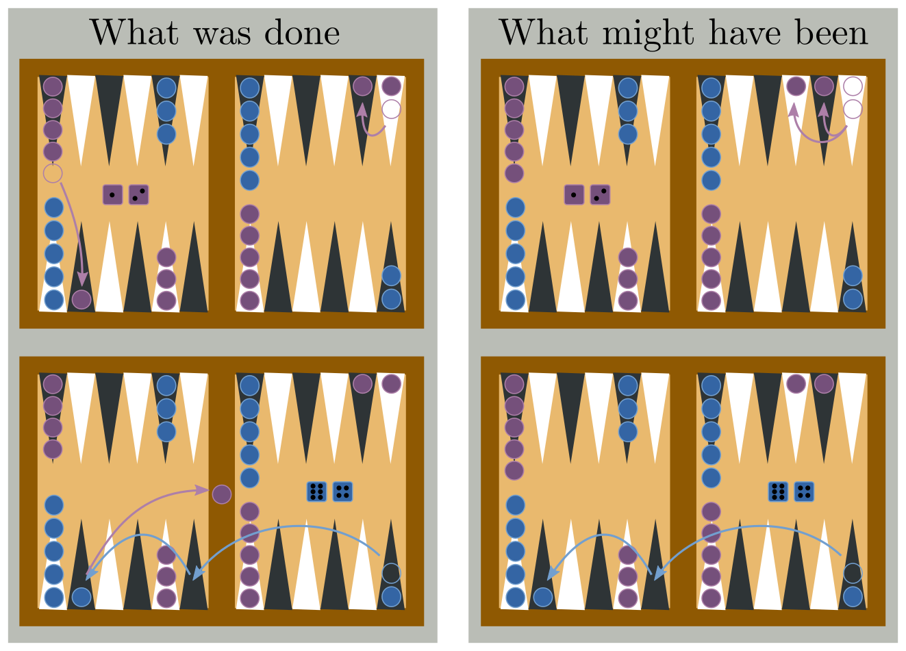
The right column of the above figure plays out an alternate scenario: you might reason counterfactually that there was a better way to play your ⚁⚀ [2,1] that wouldn't have led to you being captured (or, at least if blue still captures, not as much ground has been lost). Counterfactual reasoning leads to some regret about the choice you made. But what will you do next time? You had no way of knowing that your opponent would roll ⚅⚃ [6,4]. Next time, you won't have knowledge of their roll either. Next time, you should act exactly as you did this time. Sometimes we're unlucky, but that doesn't necessarily mean we made the wrong choice!

I conclude that for planning and learning, again all we need are interventions, not counterfactuals. (Caveats explored below in point #4).

3. Counterfactuals help learn the correct SCM

I'll keep this section short. In Elements, the authors seem to foreshadow in the early chapters that SCMs can, in fact, be falsified by later getting new data that reveals something you didn't know before, like the value of η or the fact that some variable had been intervened on. Given Pearl's emphasis on the difference between CBNs and SCMs (Rung 2 and Rung 3), when I read this I made an abductive leap and concluded that counterfactuals can be used to falsify an SCM. I imagine other readers might make the same leap. But this doesn't quite follow, does it?

Saying that you can falsify an SCM (above and beyond the interventionally equivalent CBN) is not the same as saying that counterfactuals are useful. The reasoning behind any such falsification would be based on things that have been observed, whether they were observed "then" or revealed later. We can never directly observe how things might have otherwise been. We learn the correct SCM by careful observation, interventions, and assumptions about mechanisms and functional forms. Chapter 7 of Elements is a catalog of the kinds of mechanistic assumptions you can make to make the SCM identifiable.

4. Counterfactuals overcome model-mismatch in reinforcement learning

The above examples of Alice's Cookie and the game of Backgammon both assume a world full of perfectly rational, unbounded agents. I assumed Alice can predict Bob's behavior so precisely, she knows exactly what the consequences of her retaliation will be. In the Backgammon example, I assumed your mental model faithfully simulates possible die rolls, and that you know exactly the play style of your opponent. The jargon-y way to say this is that I assumed no model-mismatch.

Interesting things happen to probabilities when there is model-mismatch. I dedicated most of a long post to it (recommended reading, of course). Intuitively, it means that what we expect to happen in the future (the prior) will be less accurate than what our experience tells us did happen (the posterior). Again using some jargon, when there is model-mismatch the average posterior is no longer equal to the prior. To say it more poetically, Truth is stranger than Fiction.

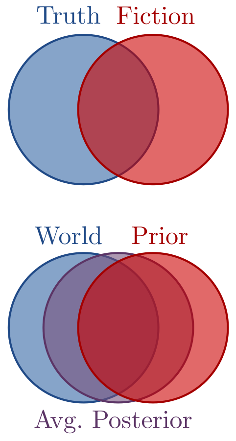
One possible, though not very effective way to learn a new skill -- or for a reinforcement learning agent to solve a task -- is by closing your eyes and simulating possible future outcomes in your mental model. These are interventional predictions and they are an exercise in imagination -- fictions. When we imagine possible future worlds, there is a lot that our imaginations get right, but there is also plenty that it gets wrong. Sometimes Truth is stranger than Fiction; other times, Fiction is stranger than Truth. The more they overlap, the better you can learn from mental simulation, or samples from the prior alone.

Fiction that is grounded in experience is closer to reality. Mathematically, we might say that posteriors drawn from experience are closer to the "world" distribution than the prior was. Instead of closing your eyes and imagining a fresh new scenario, a more effective way to learn is to pull up episodic memories of past experiences. In the analogy, memories are posteriors. The analogy I hope to drive home is that Interventions are to Priors as Counterfactuals are to (Average) Posteriors. The latter will be closer to the "true" distribution whenever there is model mismatch.

The upshot for Reinforcement Learning is that agents in nontrivial scenarios always have model-mismatch. The world can be complicated. Counterfactuals will help them learn the right policy. But before you say "episodic memory is just replay, and we already knew that!" let me add one final twist.

Replay is where the agent logs its experiences in memory and continues to revisit those memories when training its policy. The problem is, standard replay is model-free. The experience is played and re-played over and over, exactly as it happened, because in the absence of a model there's no ability to generalize to "nearby" possible worlds. Counterfactual replay is stronger. Importantly, when we reason counterfactually we don't just replay our memories "as is," but we elaborate on them, imagining plausible ways that things might have been slightly different.

Ideally, our RL agents should be able to fail but recognize that they made the right choice, or succeed but recognize they made the wrong one. That is, they should learn from near-successes and near-misses. Learning from near-successes, for instance, means that things went poorly, but you recognize that the right choice was made. This requires imagining possible alternatives -- counterfactuals -- and realizing that 9 times out of 10 things would have gone better. Just as in the Backgammon case above, sometimes you make the right choice but get unlucky. Counterfactual replay can attribute a failure either to your actions, in which case a correction to the policy is needed, or to the "noise," in which case the error results in no change to behavior. An agent who uses this kind of reasoning ought to be able to learn more quickly than one who always takes their experiences "as is."

I conjecture that there's a nice analytic result available here: an RL agent with counterfactual replay should provably learn with better data efficiency (less experience) than (i) standard replay and (ii) interventions (i.e. forward planning) alone. Further, the performance gap should grow with model-mismatch. For now, I leave this as an open problem for the reader or for a future version of myself.

Summary

1. I started with a reminder that graphs theory and probability theory are distinct, to help motivate some of the definitions in Elements.
2. I gave a non-technical introduction to the rungs of the causal ladder: association, intervention, and counterfactuals, and (hopefully) explained why each one requires more assumptions than the previous level
3. I graphically illustrated the problem of interventional equivalence of SCMs, once with discrete variables and once with continuous. This helps motivate chapter 7 of Elements which describes how to learn an SCM via making additional assumptions.
4. The practical utility of counterfactual reasoning is subtle. I ruled out three of the common defenses of counterfactuals, or at least (I hope) made it clear that they're special cases of "model mismatch," which is the only valid justification for counterfactuals that I'm aware of.

Footnotes

1. If you've tuned into any discussions on causality, you may have heard the terms "do calculus" and "do operator." The discussion now is about the do-operator. The do-calculus is a set of rules for manipulating the underlying graph (e.g. deleting an arrow) as a way to evaluate the result of the do-operator. More on this below.
2. I chose the example of Backgammon here since it is a well-known game that involves a good deal of both strategy and luck. My original example was with Chess, but I cut it since it invites the question of why a deterministic strategy game should involve probabilities in the first place. An interesting topic, no doubt, but at this point just a distraction!
3. The standard response I hear to this problem is that counterfactuals are useful for assigning blame, for instance in the legal system. When someone (or something) is demonstrably the cause of another's grievance, the legal system steps in to punish the wrongdoer. Further, such causal reasoning is clearly couched in the language of counterfactuals ("such and such grievance would not have happened if not for the actions of so and so person" implies guilt of that person), as Pearl is always quick to point out. So, counterfactuals are clearly "useful" in the credit/blame sense. THAT BEING SAID, this argument really just begs the question, "what is the utility of blame?" What's done is done. If the answer is "to disincentivize further wrongdoing, then the task once again becomes a matter of reasoning about the future, which is the purview of interventions. The true utility of counterfactuals is nontrivial and non-obvious. The last section of this post (connecting to reinforcement learning) will, I hope, make all of this clear.